Solid mechanics · analytical simulation
Cantilever Beam Mechanics
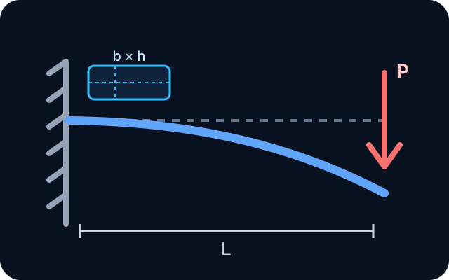
Inspect how material stiffness, beam dimensions and a free-end point load change deflection, internal forces and elastic bending stress in the public MATLAB example.
Interactive analytical model
Cantilever beam lab
Explore the rectangular Euler–Bernoulli beam encoded in the public MATLAB file. The source preset is 210 GPa, 0.75 m × 20 mm × 15 mm and a 20 N downward free-end load.
Control ranges are browser-demo bounds. The equations assume a prismatic rectangular beam, linear elasticity, small deflection and a point load at the free end; they do not check yielding, shear deformation or buckling.
Second moment I
5.625e-9 m⁴
b h³ / 12
Tip deflection
-2.381 mm
signed downward
Fixed-end moment
-15.000 N·m
source sign convention
Max outer-fibre stress
20.000 MPa
at the fixed support
- Deflection
- -0.744 mm
- Moment
- -7.500 N·m
- Shear
- 20.000 N
- Top stress
- 10.000 MPa
| x [m] | v [mm] | M [N·m] | Q [N] | |σ|max [MPa] |
|---|---|---|---|---|
| 0.000 | 0.000 | -15.000 | 20.000 | 20.000 |
| 0.188 | -0.205 | -11.250 | 20.000 | 15.000 |
| 0.375 | -0.744 | -7.500 | 20.000 | 10.000 |
| 0.563 | -1.507 | -3.750 | 20.000 | 5.000 |
| 0.750 | -2.381 | 0.000 | 20.000 | 0.000 |
Corrugated Digital Twin · source-bounded paper audit
The published test bench is a different mechanical case
The paper reports a physical corrugated-board test, a digital asset and a regression step. This panel makes that evidence chain inspectable without presenting the live cantilever calculator above as the paper's experiment, dashboard or Digital Twin.
Evidence state
Paper evidence only
No data or asset replay
1. Physical asset
Corrugated specimen in a three-point-bending test bench.
2. Measured response
Load sensing captures the specimen response and loading-history sensitivity.
3. Digital asset
A MATLAB representation and dashboard participate in bidirectional data flow.
4. Reported estimate
Linear regression estimates a displacement limit from the measured response.
| Aspect | Live beam lab above | Published Digital Twin case |
|---|---|---|
| Mechanical boundary | Fixed cantilever with a free-end point load. | Physical three-point-bending test bench. |
| Evidence class | Executed analytical Euler–Bernoulli calculation. | Physical test, Digital Twin prototype and regression reported by the paper. |
| Inputs | Editable E, L, b, h and load P with explicit SI units. | Measured response and a sensor/control protocol; no reusable export is embedded here. |
| Outputs shown here | Deflection, moment, shear and elastic bending stress. | Source evidence only; no sensor replay, MATLAB dashboard or regression result is reproduced. |
Rights boundary: All rights reserved; no reuse without permission. No paper figure, measured data or dashboard asset is copied.
Reproduction blocker: The public paper does not grant reuse rights for its assets, and no reusable sensor data, control protocol or source package has been verified.
Decision: Keep the current calculator separate; reproduce the digital-twin case only from an authorized data/protocol export.
Jason E. Djajasaputra and Ricardo Fitas. Authorea preprint v1, posted 11 December 2024. Physical test, digital-twin prototype and regression. This audit records the published case; it does not reproduce or validate its results.
Model, equations and limits
The public source defines a 210 GPa rectangular cantilever, 0.75 m long, 20 mm wide and 15 mm high, with a signed −20 N tip load. This page presents the same case as a positive 20 N downward load and preserves the source sign convention for deflection and moment.
- I = b h³ / 12 and v(x) = −P x²(3L−x)/(6EI).
- M(x) = −P(L−x), Q = P and σ = −My/I.
- The source preset gives −2.381 mm tip deflection and 20.000 MPa maximum outer-fibre stress at the fixed support.
- Outputs are analytical Euler–Bernoulli calculations, not experimental measurements or a finite-element validation.