Dynamics & vibration

Machine Dynamics & Vibration Simulations

Inspect four linear vibration models with explicit SI units: three reconstructed from Ricardo Fitas’s public MATLAB sources, plus a separately labelled 2DOF quarter-car benchmark driven by a calculated road input. Each model states its provenance and validation boundary.

Original conceptual illustration by Ricardo Fitas; not a measured or benchmark result.

Interactive analytical model

Single-degree-of-freedom vibration lab

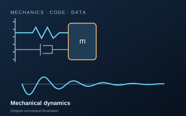
Explore the public-source equation m ẍ + c ẋ + k x = 0. The preset reproduces the parameters in Ex2.m.

MasskgStiffnessN/mViscous dampingN·s/mInitial displacementmmInitial velocitym/sDurations

Control limits are conservative browser-demo bounds, not a claimed validity envelope for every physical system. The model assumes constant linear coefficients, viscous damping, free vibration and no external force.

Regime

Underdamped

ζ = 0.000

Natural frequency

1.299 Hz

ωₙ = 8.165 rad/s

Critical damping

12247 N·s/m

c₍crit₎ = 2√km

Peak in window

10.00 mm

Analytical samples

Calculated analytical motion of the public linear mass–spring–damper model. Displacement is visually amplified to at most ±72 px; the displayed millimetres and velocity are the computed values.

Simulation time0.000 s

x(t): 10.000 mm
ẋ(t): 0.0000 m/s

Analytical free response of the linear single-degree-of-freedom model. This is a parameterized simulation, not an experimental measurement.

Independent numerical check

A fourth-order Runge–Kutta integration with 817 steps is compared with the analytical displacement at every step.

Pass · maximum |xₐₙₐₗᵧₜᵢ꜀ − xᴿᴷ⁴| = 6.59e-6 µm

Acceptance tolerance: max(0.01% of plotted peak, 0.01 µm).

Source model · Ex4 / Ex5

Two-degree-of-freedom heave–pitch lab

A rigid body is supported by front and rear linear spring–damper pairs and excited by a harmonic force at an editable offset. The calculation preserves the public MATLAB mass, damping and stiffness matrices; it is not a quarter-car model and has no wheel, tyre or road-input dynamics.

Body mass1000 kgPitch inertia1000 kg·m²Front stiffness60000 N/mRear stiffness60000 N/mFront damping100 N·s/mRear damping100 N·s/mForce amplitude2000 NForce offset1.6 mExcitation frequency10 rad/sInitial heave100 mmInitial pitch0 mradDuration8 s

Rigid-body heave and pitch calculated from the source matrices. Heave is visually amplified to ±42 px; pitch uses the calculated angle. Wheels are positional symbols only: this source model has no wheel masses or tyre stiffness.

RK4 integration of Mq̈ + Cq̇ + Kq = [F, rF]ᵀ cos(ωt). Curves use separate, labelled vertical scales.

Time cursor: 0.000 s

Current state

z 100 mm

φ 0 mrad

Calculated rates

ż 0.0000 m/s

z̈ -10.0000 m/s²

Undamped modes

f₁ 1.743 Hz

f₂ 4.359 Hz

Independent checks

Δz 1.54e-3 mm

Δφ 3.53e-3 mrad

The frequency-domain dynamic-stiffness check gives steady amplitudes of 99.5037 mm and 4.9222 mrad at the selected ω. The time trace also contains the initial-condition transient. RK4 convergence compares 801 and 1,601 time samples.

Independent calculated benchmark

2DOF quarter-car road response

A coupled sprung-mass and unsprung-mass model integrated in the browser with fixed-step RK4. A smooth raised-cosine road bump drives the tyre; the body, wheel, diagram and three plots all use the same calculated state. This is not a reproduction of the public Ex6.m, whose published ODE call uses zero external force.

Model and road input

Sprung masskgUnsprung masskgSuspension stiffnessN/mSuspension dampingN·s/mTyre stiffnessN/mBump heightmmBump lengthmVehicle speedm/sDurations

Time cursor: 0.000 s

Displacement (mm)bodywheelroad

Velocity (m/s)bodywheel

Acceleration (m/s²)bodywheel

Calculated state and response envelope
Quantity	At cursor	Peak absolute
Body displacement	0.000 mm	21.031 mm
Wheel displacement	0.000 mm	59.588 mm
Body acceleration	0.000 m/s²	6.712 m/s²
Wheel acceleration	0.000 m/s²	70.963 m/s²
Suspension travel zₛ−zᵤ	0.000 mm	50.883 mm
Tyre deflection zᵤ−zᵣ	0.000 mm	17.624 mm

Equations, boundaries and checks

mₛz̈ₛ + cₛ(żₛ−żᵤ) + kₛ(zₛ−zᵤ) = 0

mᵤz̈ᵤ − cₛ(żₛ−żᵤ) − kₛ(zₛ−zᵤ) + kₜ(zᵤ−zᵣ) = 0

Zero initial displacement and velocity; linear suspension spring/damper and linear tyre; no static sag, gravity, tyre damping, stops or nonlinear contact. The road is flat except for one raised-cosine bump beginning at 0.5 s.

Undamped body mode: 1.081 Hz
Undamped wheel-hop mode: 11.117 Hz
RK4 body Δ (1201↔2401): 5.26e-5 mm
RK4 wheel Δ (1201↔2401): 9.49e-4 mm
Linearity residual: 0.00e+0 mm

Model quarter-car-rk4-v1. Numerical checks compare the displayed 1201-sample response with a 2401-sample run and verify proportional response to bump height.

Source-derived forced response

Rotating-unbalance frequency response

Explore the stationary response encoded in the public MD1.m model. It treats the bar and motor as one rotational degree of freedom driven by an eccentric mass.

Damper position amFrequency ratio βω / ωₙ

The bounds reproduce the source scans: a = 0.1–0.7 m and β = 0–4. This is a linearized, stationary harmonic simulation. It is neither a transient solution nor experimental validation.

Damping ratio

ζ = 0.0292

cₑq = 0.998 N·m·s/rad

Motor speed

314.4 rpm

ω = 32.927 rad/s

Tip amplitude

12.975 mm

steady-state magnitude

Phase lag

90.0°

atan2(cₑqω, kₑq − Jω²)

Forcing phase cursor0° · t = 0.00000 s

Bar angle θ0.000 mrad

Tip displacement0.000 mm

Angular velocity0.5975 rad/s

Angular acceleration-0.000 rad/s²

Source-derived one-degree-of-freedom steady-state response. The replay is slowed to one cycle per four seconds for inspection; the displayed phase, physical time and SI values remain calculated from the selected ω.

One calculated steady-state cycle. The gold cursor drives the bar, motor orbit and numeric state above.

Steady-state amplitude at the bar tip. The yellow marker follows the selected frequency; the curve rescales when the damper position changes.

Source calibration

J equivalent: 0.519816 kg·m²
ωₙ: 32.9275 rad/s
kₑq: 563.595 N·m/rad
c at a = 0.1 m: 0.998 N·m·s/rad
High-β limit: 0.75652 mm

Damping and stiffness are reconstructed from the source’s eleven decay peaks, 0.1909 s damped period and stated geometry. Values are computed in the browser, not copied from a chart.

Computed forced response at selected frequency ratios
β	rpm	X [mm]	M₀ [N·m]	F spring [N]	F damper [N]
0.500	157.2	0.252	0.1491	0.397	0.058
1.000	314.4	12.975	0.5963	20.455	5.963
2.000	628.9	1.008	2.3853	1.589	0.926
4.000	1257.7	0.807	9.5411	1.272	1.483

Independent equation check

The implementation evaluates the complex dynamic stiffness |kₑq − Jω² + i cₑqω|. The build validator independently compares it with the normalized amplification equation, checks the a² damping law, zero-speed response, the 0.75652 mm high-frequency asymptote and the phase replay residual Jθ̈ + cₑqθ̇ + kₑqθ − M₀cos(ωt).

Model and provenance

The public Ex2.m script defines the free translational model; Ex4.m and Ex5.m define the two-degree-of-freedom heave–pitch matrices and harmonic point force. A second public source, MD1.m, defines the equivalent rotational inertia, geometry, decay calibration and stationary response to rotating unbalance. Those three labs preserve the source models. The quarter-car lab is an independent linear benchmark added to make a road input physically coupled and inspectable; it is not attributed to the public MATLAB files. None of the browser output is presented as experimental data.

Mass m in kg, stiffness k in N/m and damping c in N·s/m.
Initial displacement x(0) in m and velocity ẋ(0) in m/s.
Closed-form solutions for underdamped, critical and overdamped regimes.
Complex dynamic-stiffness solution and synchronized steady-state phase replay for the forced rotational response.
Two-degree-of-freedom rigid-body response with front/rear support asymmetry and harmonic force offset.
Independent 2DOF quarter-car response to a raised-cosine road bump, with synchronized body, wheel and road states.
CSV export contains the analytical time, displacement and velocity series in SI units.

Complete public-source inventory

MATLAB models and current coverage

Inventory of every pertinent top-level calculation in the two public MIT repositories at commits 9d458050 and a97995a4. Drawing helpers and generated Simulink caches are grouped with their parent model.

Source	Physical model	ProjectHub state	Evidence boundary
Ex1 / Ex2 / Ex2_9 / Ex_2_10	Undamped/damped translational SDOF; symbolic, analytical, ODE and Simulink forms	Calculated and validated	Browser analytical solution plus independent RK4; Simulink binary is not executed.
Ex4 / Exercise_4_2	Free rigid-body heave and pitch with two spring–damper supports	Calculated in this page	Same 2×2 matrices; bounded RK4, synchronized body and curves.
Ex4_4	Front/rear damping parameter fit	Source identified	Optimization surface is not yet reproduced; objective mixes heave and pitch sums.
Ex5 / Ex5_2	Harmonic point-force transient and frequency response	Calculated in this page	Time integration plus independent complex dynamic stiffness at selected ω.
Ex5_3	Force-position and damping optimization	Source identified	No optimizer shown until bounds and the mixed-unit objective are reviewed.
Ex6	Road-profile animation intent	Source gap retained; independent benchmark above	The published ODE call passes zero external force; the sinusoidal road is drawn but not coupled. The quarter-car lab above is explicitly independent.
MD1	Rotating unbalance of a bar–motor assembly	Calculated and validated	Complex dynamic stiffness, decay calibration, asymptotic checks and equation-checked phase replay.