Finite elements · structural mechanics · heat transfer

Finite Element Engineering Applications

Solve the public MATLAB fin problem with linear one-dimensional elements, inspect its assembled temperature field and compare every node with the independent insulated-tip analytical solution.

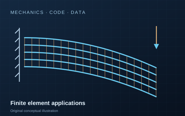
Original conceptual illustration by Ricardo Fitas; not the thermal mesh or a measured result.

Executed browser FEM · independent demo

2D plane-stress cantilever

linear elasticityT3 / CSTsmall strainnot a paper replay

MeshT3Young's modulusGPaEnd loadN ↓Deformation scale××250

Mesh

128 T3

85 nodes

Tip uy

-0.1947 mm

mean end edge

Max |u|

0.1968 mm

nodal magnitude

Max von Mises

11.612 MPa

element constant

Force balance

8.96e-10 N

ΣRy + ΣFy

T3/CST mesh · plane stress · SI calculation · deformation amplified ×250. Field range: 0–0.197 mm.

Mesh convergence · mean end-edge uy
Mesh	T3	uy [mm]	EB difference
8 × 2	32	-0.1228	48.43%
16 × 4	128	-0.1947	18.23%
20 × 5	200	-0.2099	11.84%

Geometry: 1.00 × 0.20 × 0.010 m
Poisson ratio: 0.30
Reaction Ry: 1.000e+3 N
Reaction Mz: 1.000e+3 N·m
Strain energy: 0.097 J

EB reference uy: 0.2381 mm
Reference difference: 18.23%
Element: linear T3 / CST
Constitutive model: isotropic plane stress
Model version: cst-cantilever-v1

Executed browser FEM · source preset

Steady fin heat-transfer lab

Assemble and solve the same linear-element conduction and distributed-convection system declared in FEM2.m. Width remains at the source value of 1 m; the natural right boundary is an insulated tip.

Linear elementscountConductivity kW/(m·K)Convection hW/(m²·K)Fin length LmThickness tmmBase temperature°C

Browser bounds are demonstration limits. The source assumptions are steady one-dimensional conduction, constant properties, uniform cross-section, prescribed base temperature, distributed lateral convection and zero tip heat flux.

Mesh

8 elements

9 nodes · Δx 12.50 mm

Insulated-tip temperature

190.494 °C

analytical 190.518 °C

Base heat rate

333.706 W

analytical 333.517 W

Independent check

0.0240 °C

max nodal · 0.056% heat rate

Calculated piecewise-linear temperature field. Gold arrows denote distributed lateral convection; colour is normalized between ambient and base temperature for the current case.

Blue nodes and segments are the assembled finite-element solution. The dashed gold reference is the independent closed-form insulated-tip fin solution.

Inspect node

Position: 0.10000 m
FEM: 190.4941 °C
Analytical: 190.5181 °C
Signed error: -0.02396 °C

Finite-element and analytical temperatures at every mesh node
Node	x [m]	FEM [°C]	Analytical [°C]	Error [°C]
0	0.00000	235.0000	235.0000	-0.00000
1	0.01250	224.2397	224.2457	-0.00601
2	0.02500	215.0786	215.0896	-0.01102
3	0.03750	207.4451	207.4603	-0.01511
4	0.05000	201.2795	201.2978	-0.01837
5	0.06250	196.5333	196.5542	-0.02085
6	0.07500	193.1695	193.1921	-0.02259
7	0.08750	191.1617	191.1853	-0.02362
8	0.10000	190.4941	190.5181	-0.02396

Source audit and evidence boundary

The MIT-licensed public repository contains two MATLAB heat-transfer scripts and an Abaqus folder. FEM2.m supplies the dimensions, material and convection values, linear-element matrices, a prescribed 235 °C base and a natural insulated tip. This browser calculation reimplements that declared system; it is not a recording or an Abaqus execution.

The governing steady fin equation is kA T″ − hP(T−T∞) = 0.
Each element uses the source conduction matrix and consistent convection matrix/load; the base temperature is enforced exactly.
The comparison uses θ(x)=θb cosh[m(L−x)]/cosh(mL), with m²=hP/(kA).
No Code_Aster or SALOME-MECA case exists in the public tree. The Abaqus geometry is stored in a binary CAE file; no reusable ODB/mesh/field export is present, so this page does not claim an Abaqus replay.